3D Spherical Overpressure
This test illustrates the ability of a code to handle a spherical explosion due to spherical overdensity and overpressure. The test consists of a sphere of radius 0.2 centered at (0.5, 0.5, 0.5) with a density of 1 and pressure of 11, surrounded by a background density and pressure of 0.1 and 1, respectively. This test was performed with the default hydro build (cholla/builds/make.type.hydro) and Van Leer integrator. Full initial conditions can be found in cholla/src/grid/initial_conditions.cppunder Spherical_Overpressure_3D().
Note that the output directory needs to be changed for the user.
#
# Parameter File for the 3D Sphere Overpressure.
#

######################################
# number of grid cells in the x dimension
nx=256
# number of grid cells in the y dimension
ny=256
# number of grid cells in the z dimension
nz=256
# output time
tout=0.1
# how often to output
outstep=0.01
# value of gamma
gamma=1.66666667
# name of initial conditions
init=Spherical_Overpressure_3D
# domain properties
xmin=0.0
ymin=0.0
zmin=0.0
xlen=1.0
ylen=1.0
zlen=1.0
# type of boundary conditions
xl_bcnd=1
xu_bcnd=1
yl_bcnd=1
yu_bcnd=1
zl_bcnd=1
zu_bcnd=1
# path to output directory
#outdir=/gpfs/alpine/scratch/bvilasen/ast149/sphere_explosion/output_files/
outdir=/raid/bruno/data/cosmo_sims/cholla_pm/sphere_explosion/
Upon completion, you should obtain 11 output files. The initial and final densities and pressures (in code units) of a slice along the y-midplane is shown below. Examples of how to plot projections and slices can be found in cholla/python_scripts/Projection_Slice_Tutorial.ipynb.
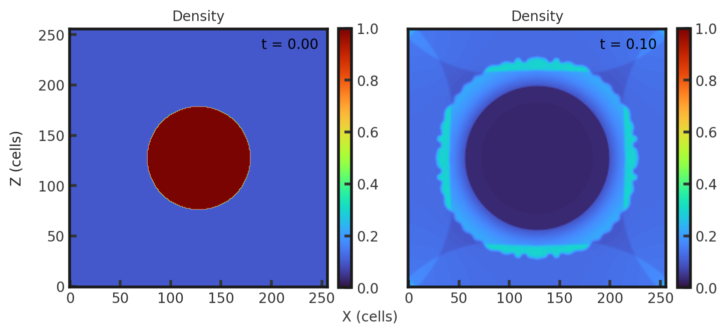
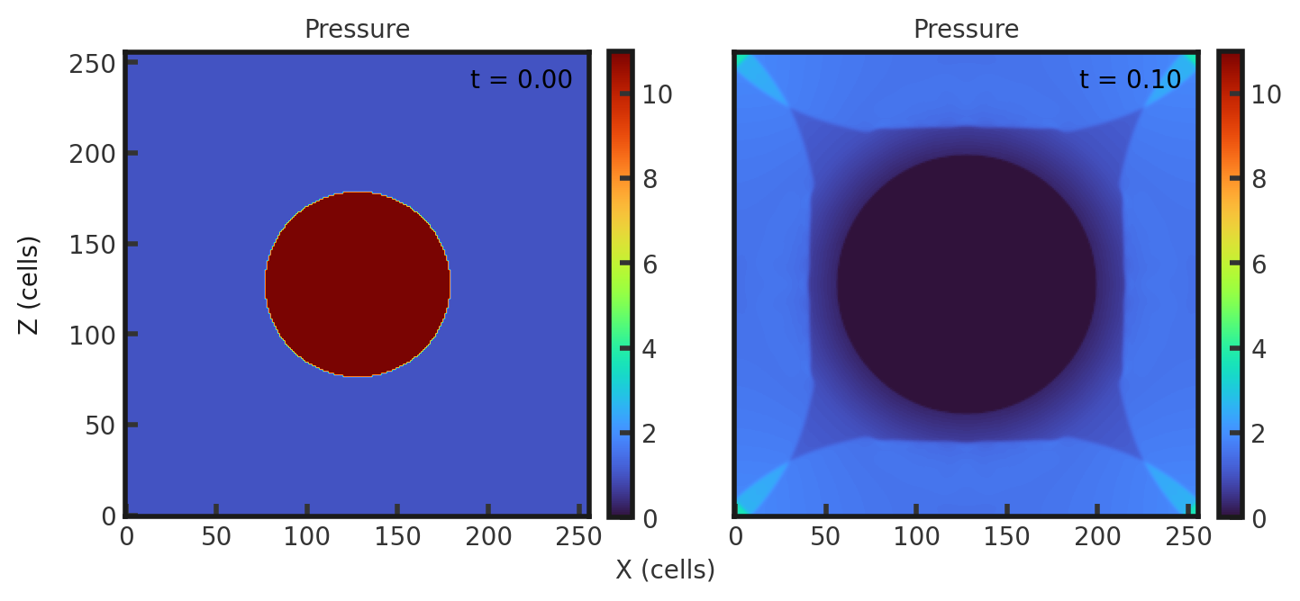
Currently (8/1/23) this test is producing identical solutions regardless of whether the default hydro or gravity build is used. The sphere has exploded, leaving an area of low density and pressure in place of the original higher density and pressure sphere. Spherical symmetry is strongly preserved, with the final density having circularly symmetric perturbations ringing the newer area of high density.