Skip to content
evazlimen edited this page Jul 22, 2024 · 2 revisions

1D Shu and Osher test

This test (Shu & Osher, 1989) highlights the ability of a code to resolve small scale smooth flow and shocks simultaneously. Further, it shows how lower resolution solutions can cut off some of the amplitude of maxima due to the slope limiters. Parameters are from Stone et al., 2008, Section 8.1. The test consists of left and right states separated at x = -0.8. On the left, density is set to 3.857143, pressure to 10.33333, and velocity to 2.629369. On the right, density is sinusoidally varying: $\rho(x)$ = 1.0 + 0.2 $\sin(5.0\pi x)$. Pressure is set to 1.0 and the velocity is 0.0. Gamma is set to 1.4. This test is performed with the hydro build (cholla/builds/make.type.hydro). Full initial conditions can be found in cholla/src/grid/initial_conditions.cppunder Shu_Osher().

Important: This test must be run with diode boundaries disabled in order to perform as expected (thank you @alwinm!). This branch also uses the Van Leer integrator.

Parameter file: (modified from cholla/examples/1D/Shu_Osher.txt)

Modified to add yl_bcnd, yu_bcnd, zl_bcnd, and zu_bcnd=0. Xmin changed to -1.0 and xlen to 2.0.

# Parameter File for the Shu-Osher shock tube test, originally from
#     Shu & Osher, 1989. These parameters are from Stone et al., 2008, Section 8.1
#

######################################
# number of grid cells in the x dimension
nx=200
# number of grid cells in the y dimension
ny=1
# number of grid cells in the z dimension
nz=1
# final output time
tout=0.47
# time interval for output
outstep=0.47
# value of gamma
gamma=1.4
# name of initial conditions
init=Shu_Osher
# domain properties
xmin=-1.0
ymin=0.0
zmin=0.0
xlen=2.0
ylen=1.0
zlen=1.0
# type of boundary conditions
xl_bcnd=3
xu_bcnd=3
yl_bcnd=0
yu_bcnd=0
zl_bcnd=0
zu_bcnd=0
# path to output directory
outdir=./

Upon completion, you should obtain 2 output files. The initial and final density, pressure, and velocity (in code units) of the solution is shown below (pink dots) plotted over high resolution solution with 4000 cells (purple line). Examples of how to extract and plot data can be found in cholla/python_scripts/plot_sod.ipynb.
Three rows of two scatter plots side by side. The first row shows density vs x position, with the leftmost plot showing the initial and the rightmost the final. The second and third rows are the same for pressure and velocity, respectively. The first column is plotted with pink dots while the second has pink dots plotted over a purple line. In all cases, the pink dots follow the shape of the purple line. In the upper right hand corner is the text 't= 0.00' for all the plots in the first column and 't= 0.47'for all the plots in the second column. The initial density plot (row 1 column 1) has a value of 3.857143 for x <-.8 and a sine wave of 1 + .2sin(5.0*pi*x) for all other x. The final density plot has a constant value of 3.857143 from x = 0 to x = -0.5 and a slanted, slightly irregular wave until x = .45. This wave oscillates between 4 and 3.5 and is leaning to the left. At x = .45, the wave begins to break down and become more erratic, lastly dropping to a value of around 1 for x = .8-1.0. For the pressure plots (row 2), the initial plot has a value of 10.33333 for x <-.8 and 1 otherwise. The final plot is similar to the final density plot, with an initial value of 10.33333 from x = 0 to x = -0.5 and a slanted wave following. The wave oscillates between 11 and 9 and does not break down until x = 0.8, where it drops to a constant value of 1 for the remaining x values. The initial velocity plot shows a value of 2.629369 for x < -0.8 and 0 elsewhere. The final velocity plot looks similar to the final pressure and density, with a constant value pf 2.629369 until x = -0.5, followed by a slanted wave. However, this wave slants right instead of left and oscillates between 2.5 and 3. The wave breaks down at x = 0.8, dropping to a value of zero.

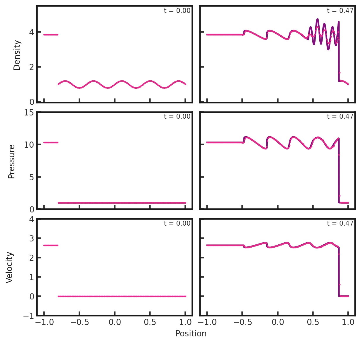
With the diode disabled, this solution does match that of Schneider and Robertson 2015 and Stone et al. 2008, shown below:

Clone this wiki locally