Skip to content
evazlimen edited this page Jul 23, 2024 · 2 revisions

3D Sod Shock Test (High resolution version)

This is a higher resolution version of the sod shock test, with a grid of 256x256x256.Parameters from Sod (1978). Illustrates the ability of a code to resolve shocks and contact discontinuities over a narrow region. The test consists of two constant states (on left pressure and density are equal to 1; on right they are equal to 0.1) separated by a discontinuity at 0.5. Gamma is set to 1.4. This test is performed with the default hydro build (cholla/builds/make.type.hydro) and Van Leer integrator.

Parameter file: (cholla/examples/3D/sod256.txt)

#
# Parameter File for 3D Sod Shock tube
#

################################################
# number of grid cells in the x dimension
nx=256
# number of grid cells in the y dimension
ny=256
# number of grid cells in the z dimension
nz=256
# final output time
tout=0.2
# time interval for output
outstep=0.2
# name of initial conditions
init=Riemann
#init=Read_Grid
# domain properties
xmin=0.0
ymin=0.0
zmin=0.0
xlen=1.0
ylen=1.0
zlen=1.0
# type of boundary conditions
xl_bcnd=3
xu_bcnd=3
yl_bcnd=3
yu_bcnd=3
zl_bcnd=3
zu_bcnd=3
# path to output directory
outdir=./

#################################################
# Parameters for 1D Riemann problems
# density of left state
rho_l=1.0
# velocity of left state
vx_l=0.0
vy_l=0.0
vz_l=0.0
# pressure of left state
P_l=1.0
# density of right state
rho_r=0.1
# velocity of right state
vx_r=0.0
vy_r=0.0
vz_r=0.0
# pressure of right state
P_r=0.1
# location of initial discontinuity
diaph=0.5
# value of gamma
gamma=1.4

Upon completion, you should obtain two output files. The initial and final densities (in code units) of a slice along the y-midplane is shown below. Examples of how to plot projections and slices can be found in cholla/python_scripts/Projection_Slice_Tutorial.ipynb.
Two 2D histograms side by side, showing density of cells in the z direction vs cells in x direction. The leftmost is the initial density plot with a constant density of 1 throughout all 256 y cells between x-cells 0 through 128 and a constant density of 0.1 between x cells 128 through 256. The rightmost plot is the final density plot at t = 0.20 with a nonconstant density in x and constant density in z. A density of 1 transitions abruptly to a density 0.8 around x = 70 cells, then gradually lessens to 0.6 around x = 125 cells. An abrupt change occurs at x = 170 cells to a density of 0.3 and the final abrupt transition is at x = 225 cells to a density of 0.2
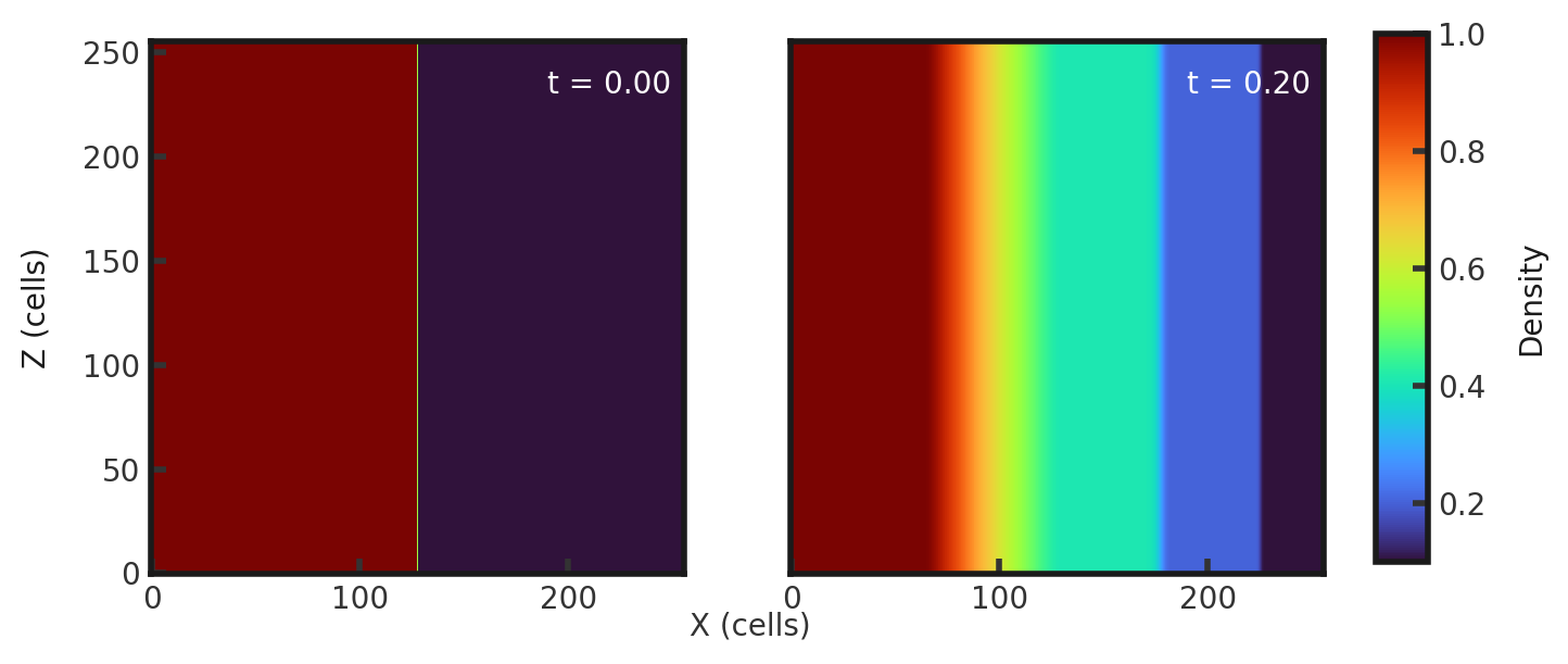
We see a smoother density gradient within the rarefaction wave due to the higher resolution. A skewer in x along the y and z midplanes yields the traditional 1-dimension solution shown below (pink dots) plotted over the exact solution (purple line).:
Two rows of two scatter plots side by side. The first row shows density vs x position while the second shows pressure vs x position. In all rows, the first plot has the text 't = 0.00' in the upper right corner while the second plot has the text 't = 0.20' in the upper right corner. The plots of the first column are shown with pink dots while the plots of the second column have pink dots plotted over a purple line. In all cases, the pink dots match the shape of the purple line, albeit imperfectly. The first plot in the first row (initial density) shows a density of 1.0 for x = 0 to x= 0.5 and a density of 0.1 for the remaining x values. The second (final density) plot shows a density of 1.0 for 0 \< x \< 0.2, then a continuous gradual decrease to a value of 0.4 at x = 0.5. Density remains constant until x = 0.7, then it jumps down abruptly to a value of 0.2. Density remains constant here until x = 0.9 where it makes a final jump to a value of 0.1, remaining at 0.1 for the final x values. In the second row, the first plot (initial pressure) is identical to the initial density plot. The second plot (final pressure) shows a pressure of 1.0 for 0 \< x \< 0.2, then a continuous gradual decrease to a value of 0.3 at x = 0.5. Pressure remains constant until x = 0.9 where it makes a jump to a value of 0.1, remaining at 0.1 for the final x values.
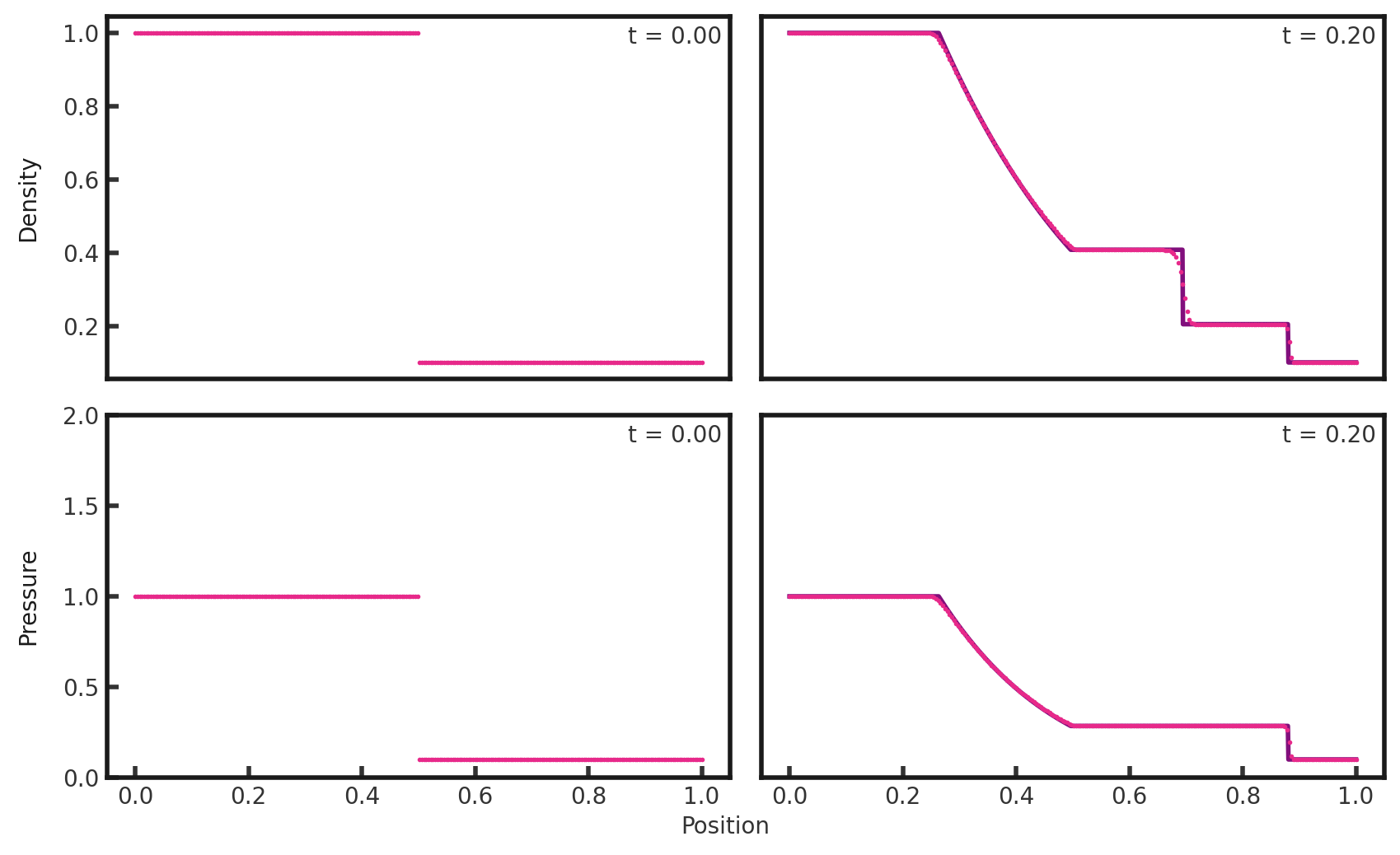
We can see a rarefaction wave on the left side, followed first by a contact discontinuity and then a shock. Transitions between shocks are resolved more narrowly.

Clone this wiki locally