Skip to content
evazlimen edited this page Jul 22, 2024 · 7 revisions

1D Blast Wave

This test is designed to assess the performance of a code near strong shocks and contact discontinuities. Parameters are derived from Woodward & Collela, 1984. The test consists of three regions. For x < 0.1, pressure is set to 1000.0. For x > 0.9, pressure is set to 100. Everywhere else, pressure is set to 0.01. Density is set to 1.0 everywhere and velocity everywhere is zero. Gamma is set to 1.4. This test is performed with the hydro build (cholla/builds/make.type.hydro) and Van Leer integrator. Full initial conditions can be found in cholla/src/grid/initial_conditions.cppunder Blast_1D().

Parameter file: (cholla/examples/1D/blast_1D.txt)

#
# Parameter File for the 1D interacting blast wave test from
#     Woodward & Collela, 1984. See also Stone et al., 2008, Section 8.1
#

######################################
# number of grid cells in the x dimension
nx=400
# number of grid cells in the y dimension
ny=1
# number of grid cells in the z dimension
nz=1
# final output time
tout=0.038
# time interval for output
outstep=0.00038
# value of gamma
gamma=1.4
# name of initial conditions
init=Blast_1D
# domain properties
xmin=0.0
ymin=0.0
zmin=0.0
xlen=1.0
ylen=1.0
zlen=1.0
# type of boundary conditions
xl_bcnd=2
xu_bcnd=2
yl_bcnd=0
yu_bcnd=0
zl_bcnd=0
zu_bcnd=0
# path to output directory
outdir=./

Upon completion, you should obtain 101 output files. The initial and final density, pressure, and velocity (in code units) of the solution is shown below (pink dots) plotted over a high resolution solution with 4000 cells (purple line). Examples of how to extract and plot data can be found in cholla/python_scripts/plot_sod.ipynb.
Three rows of two scatter plots side by side. The first row shows density vs x position, with the leftmost plot showing the initial and the rightmost the final. The second and third rows are the same for pressure and velocity, respectively. The first column is plotted with pink dots while the second has pink dots plotted over a purple line. In all cases, the pink dots follow the shape of the purple line. The initial density plot shows a constant value of one. The initial pressure plot shows a value of 1000 for x less than 0.1, 0.01 from x = 0.1 to x = 0.9, and a value of 100 from x = 0.9 to x = 1.0. The initial velocity plot shows a constant velocity of zero. The final density plot shows a curve increasing slightly from close to zero to around a value of 0.2 at x = 0.6, then jumping to a value of 2, reaching this value at x = .7. Here it jumps discontinously to 5, then decreases rapidly but continuously to 4 at x = .75 and then again to 3 at x = .78. It abruptly jumps at x = .8 to a value of 6, then jumps down to a value of 0.5. At x = .85 it jumps again to 0.2. The final pressure plot shows a curve with value of 80 increasing to 110 by x = 0.7. It then jumps discontinously to a value of 400 and then decreases smoothly until x = .8 to a value of 100. It remains at 100 until x = 0.85 at which it drops to 10. In the final velocity plot, velocity increases steadily from zero to a value of 10 at x = 0.6, where is drops discontinuously to a value of 2. It begins to increase again to a value of 13 by x = 0.85, changing slope to increase less rapidly at x = 0.75. It then drops to a value of zero, where it remains for the rest of the plot. In the upper right hand corner is the text 't= 0.00' for all the plots in the first column and 't= 0.038'for all the plots in the second column.

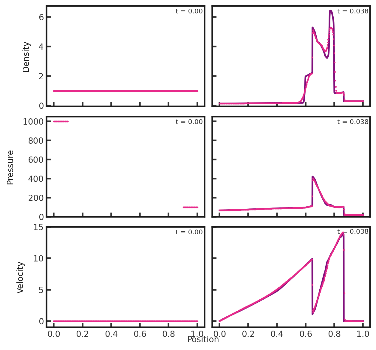
We see a contact discontinuity around x = 0.6 followed by a shock at x = 0.65 and a rarefaction fan. We have a contact discontinuity just past x = 0.75 cells and a shock at x = 0.85.

We can also obtain the evolution of the density (here at 10 fps):

Clone this wiki locally