Basic Analysis
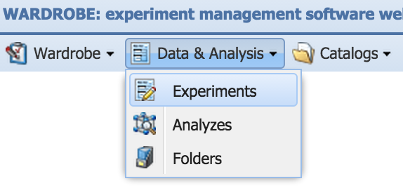
Use the Experiments window to perform basic data analysis and view the results (Data & Analysis>Experiments).
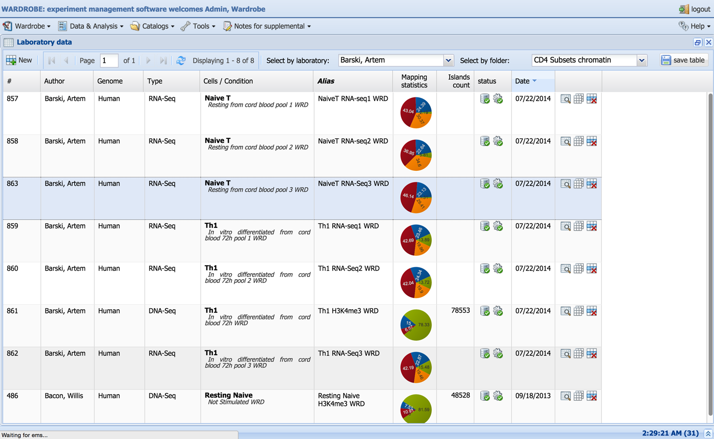
The Experiments table shows all the records created by or shared with the user’s laboratory. The datasets can be filtered by many variables, such as folder, owner and experiment type. The table shows the unique dataset identification number (“#”) and owner of the record (“Author”), description parameters (“Genome”, “Type”, “Cells/Condition”, “Alias”) and some mapping statistics in the form of a pie chart (“Mapping statistics”). Pictograms show the status of the record: downloading stage (  ,
,  ,
,  ) and processing stage (
  ,
,  ,
,  ). Please note that the status is updated every 10 minutes and that the system will not start downloading the record immediately. Depending on the number of new records entered at the same time, the records will have to wait in the queue for download or analysis.
Records can be viewed, duplicated or deleted using the three pictograms in the last column (  ,
,  ,
,  ). Unneeded records can be deleted by clicking the delete icon .
Go to Data & Analysis>Experiments.
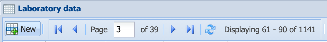
Press the “New” button in the toolbar of “Laboratory data” window.
Tip: If the record to be entered is similar to one that already exists, it can be created by clicking the “Duplicate record” icon located in the last column of the table.
Experiment form has four tabs: “General info”, “Protocol”, “Notes” and “Advanced”.
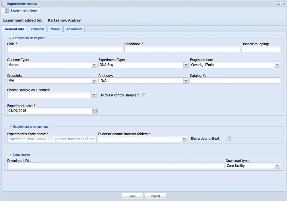
- “Experiment Description” fieldset
The following parameters in “General info” tab are needed to describe your sample: Cells, Conditions, Genome Type, Experiment Type, Fragmentation and Experiment Date. Donor field is not in use currently, but will be used for paired statistical analysis in the future.- Parameters for RNA-Seq or ChIP-Seq
- Genome Type

Select the genome to which the data will be mapped: Use the “+ spike” option only if you are using ERCC controls for RNA-Seq. - Experiment Type
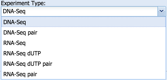
- Select DNA-Seq for ChIP-Seq, DNase-Seq, MNase-Seq and all other experiments in which the data need to be mapped to the genome; select RNA-Seq for experiments in which mapping to a transcriptome is preferred.
- Select paired-end (“pair”) or single read. If paired-end read is selected, BioWardrobe will expect to match two FASTQ files from core or one SRA from external source. If the stranded RNA-Seq protocol was used, please select “dUTP”, as this will affect RPKM calculations.
- Fragmentation
Select which fragmentation type was used for library preparation.
- Genome Type
- ChIP-Seq additional parameters
When you choose “DNA-Seq” or “DNA-Seq pair” as an “Experiment type” additional parameters will be shown.- Crosslink
- Antibody
Select your ChIP antibody or other protocol (e.g. DNaseI). This selection will affect the pipeline parameters and island calling (e.g. narrow peaks vs. broad peaks in MACS). The pipelines and parameters for each antibody can be set up in the antibody catalog by laboratory-level administrators. You can also add antibody catalog # for your records. - Background/Controls/Input
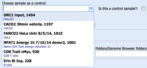
If you want MACS2 to use an input library as a control during peak calling, you can specify the control record using the drop down menu. This menu contains all samples that has been designated as controls. You can designate a sample to be used as a control using a checkmark on the right. When adding control to a record that has already been processed, remember to click the “Force to repeat analysis” checkmark on the advanced tab and click Save.
- Parameters for RNA-Seq or ChIP-Seq
- “Experiment Arrangement” fieldset:
- Experiment’s short name:
Select a short name for the experiment. This name will display on the genome browser and will be used to designate the sample during analysis. Please select a name that is UNIQUE and SHORT but DESCRIPTIVE. DO NOT use “_” or “-“ in lieu of spaces. The name can be edited after processing is complete. - Folders/Genome Browser folders:
Folders are used to organize data on the browser and to share data between laboratories. Folders can be set up and shared by laboratory-level administrators (see Wardrobe Settings section). If the folder is not selected, the data will be downloaded but not analyzed. You can only select folders that belong to or have been shared with your laboratory. The data can be moved to another folder at any time, but relocating data will affect data visibility for other laboratories. - Checking the “Share data online?” box will deposit data on the external mirror of the genome browser if it has been set up. (Normally data are deposited on the browser available only on the internal network.)
- Experiment’s short name:
- “Data Source” fieldset:
ChoData can currently be obtained from the CCHMC Core facility (CCHMC users only), the internet (a direct URL to a FASTQ or SRA file), GEO/SRA database, or a local file uploaded to the server’s shared drive (“Server upload directory”).
Also samples already in BioWardrobe can be used as a source of data.- Core facility:
Enter a filename or a code that will allow Wardrobe to find and download the file. Please note that the code needs to be unique (e.g. code such as AB1 will not work if there is also another sample named AB11). For paired-end samples, please use the common part of file name. For example, if the files are read1_bestChIP.fastq.gz and read2_bestChIP.fastq.gz, please enter “bestChIP”. - Direct link:
Please enter a URL for the file. The URL must end with the file name and extension. Wardrobe can process .fastq and .sra files that are uncompressed or compressed with .gz, .bz2, or .zip. Currently, .tgz files cannot be processed. If there are several files (e.g. sequencing data from several lanes), the URLs can be separated by semicolons (;). For paired-end data, the URLs for the first and second FASTQ should be separated by semicolons. *Currently, paired-end data coming from several lanes require manual processing. - Data already in BioWardrobe
Please put the library # in this field. *This can also be used to combine several sequencing runs. For example, to combine fastq files in records 6411, 6425, and 6470, enter “6411 6425 6470” (separated by space) in the URL field.
- Core facility:
The full instructions can be found How to upload data from GEO
You can enter protocol information and notes (including images and hyperlinks) in these tabs.
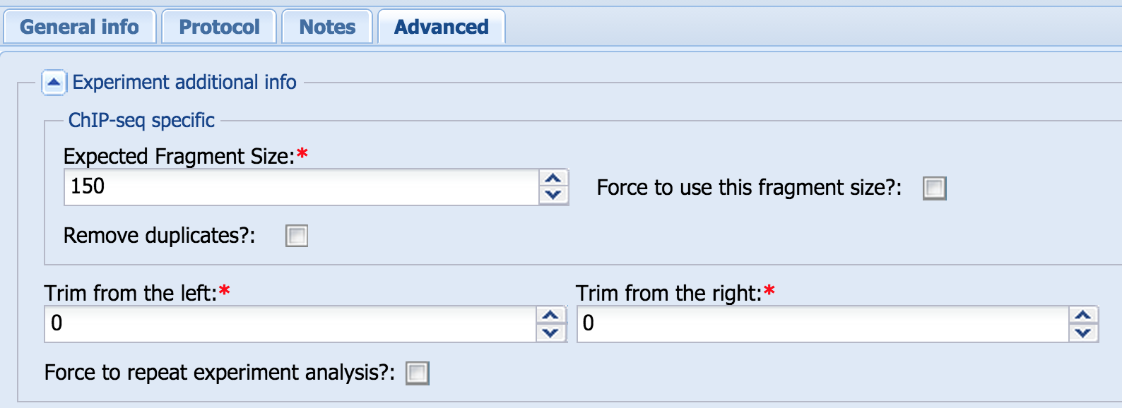
- Experiment additional info, ChIP-seq specific parameters:
Confirm or select the expected fragment size (“Expected Fragment Size”). In some cases, MACS does not determine the fragment size correctly. In these cases, you can force it to use the fragment size that you select by checking the “Force to use this fragment size?” box.
Selecting the “Remove duplicates?” box will remove coincident reads (pairs of reads that start and end at the same position on the same strand) after alignment and before analysis. - Experiment additional info common part:
Trim from the left/right:
Selecting the “Trim from the left” or “Trim from the right” options allows getting rid of sequenced indices or poor-quality bases from either end of the read.
If you change any of the advanced options after finishing the initial analysis, select the “Force to repeat experiment analysis?” box (only visible after the initial analysis) and click the “Save” button to implement these changes in the analysis.
Make and save the changes only ONCE and let the reanalysis finish before further modifying any of the options, otherwise the pipeline will break.

Quality Control Tab can be divided into three groups of information Alignment Statistics, Base frequency plot and QC plot.
For RNA-Seq type data next statistics are shown:
- the total number of reads (“Tags total”)
- the number of reads mapped in a unique fashion to transcriptome (“Tags mapped”) or genome outside of the transcriptome (“Outside annotation”)
- multi-mapped (“Multi-mapped reads”, reads which are discarded there is more than one place on the genome where read can be aligned)
- unmapped (percentage shown in red in the pie chart).
- Ribosomal contamination shows the number of reads that can be mapped to ribosomal DNA repeat. This reflects the completeness of ribosomal RNA removal during library preparation.
A high percentage of reads outside of the transcriptome (percentage shown in orange in the pie chart) may be due to DNA contamination and can inflate RPKM values by several points; this contamination is often a result of insufficient, on-column DNAse digestion.
For DNA-Seq type data the system presents statistics:
- the total number of reads (“Tags total”)
- the number of reads mapped to the genome (“Tags mapped”)
- multi-mapped (“Multi-mapped reads”, which are discarded)
- mapped duplicates (“Mapped duplicates”, which may be discarded depending on the selected settings in the Advanced tab of the Experiment form tab)
- unmapped (percentage shown in red in the pie chart).
In the case of single read sequencing fragment size is estimated by MACS (“Estimated fragment size”) from the distribution of reads mapping to the top and bottom strands.
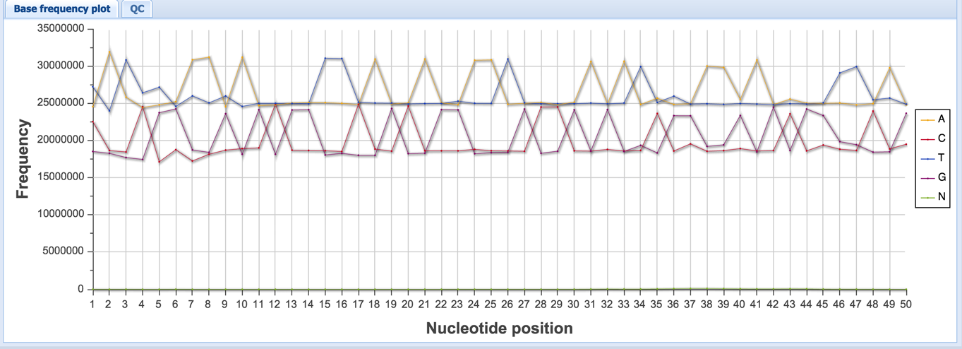
“Base frequency plot” shows how often each base is present at each position of the read. Spikiness of the base frequency plot can help detect adapter contamination during library construction. The ratio of CG/AT can also indicate the presence of DNA contamination – in the human genome, the CG/AT is ~60/40, whereas in the human transcriptome, it is closer to ~50/50.
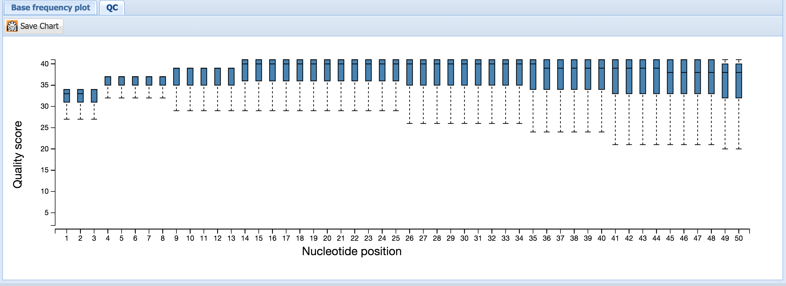
p(. The “QC” box plot shows the distribution of Phred quality scores for each base as reported in the FASTQ file.
“File link” can be used to download the read mapping data (.bam) for use in other software. The same name can be used to find the sample’s folder on the Wardrobe server.

The data are displayed on the genome browser as coverage per million reads. For single-read DNA-Seq, coverage is calculated after extending the reads to the estimated fragment size. For pair-end reads, actual fragment sizes are used. Islands identified by MACS are shown under the signal track. For RNA-Seq, actual coverage by reads is used. For stranded RNA-Seq, reads mapping to the top and bottom strand are shown separately. Please note that for the dUTP method, the reads will map to the opposite strand.
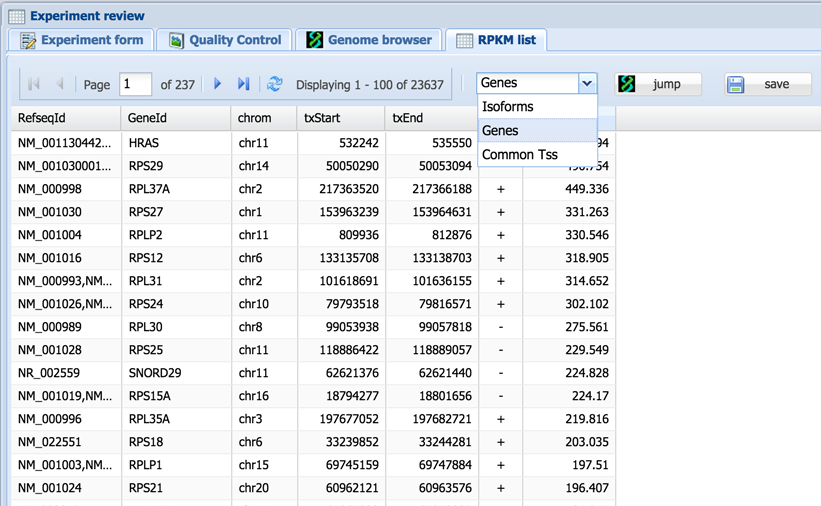
The RPKM tab displays for RNA-Seq type records and shows RPKM values for genes or isoforms. Total read number can also be shown (select the drop-down menu of one of the columns>Columns>TOT_R). Values are initially determined by our algorithm for each RefSeq by isoform; however, they can also be summed up for common TSS (for promoter activity studies, e.g. average tag density profiles) and for genes (for functional analysis, e.g. GO) using the drop-down menu.
The table can be sorted, searched and filtered by clicking on the appropriate column headings. The “Jump” button opens the genome browser tab on the selected gene. The “Save” button allows the table to be downloaded in .csv format.
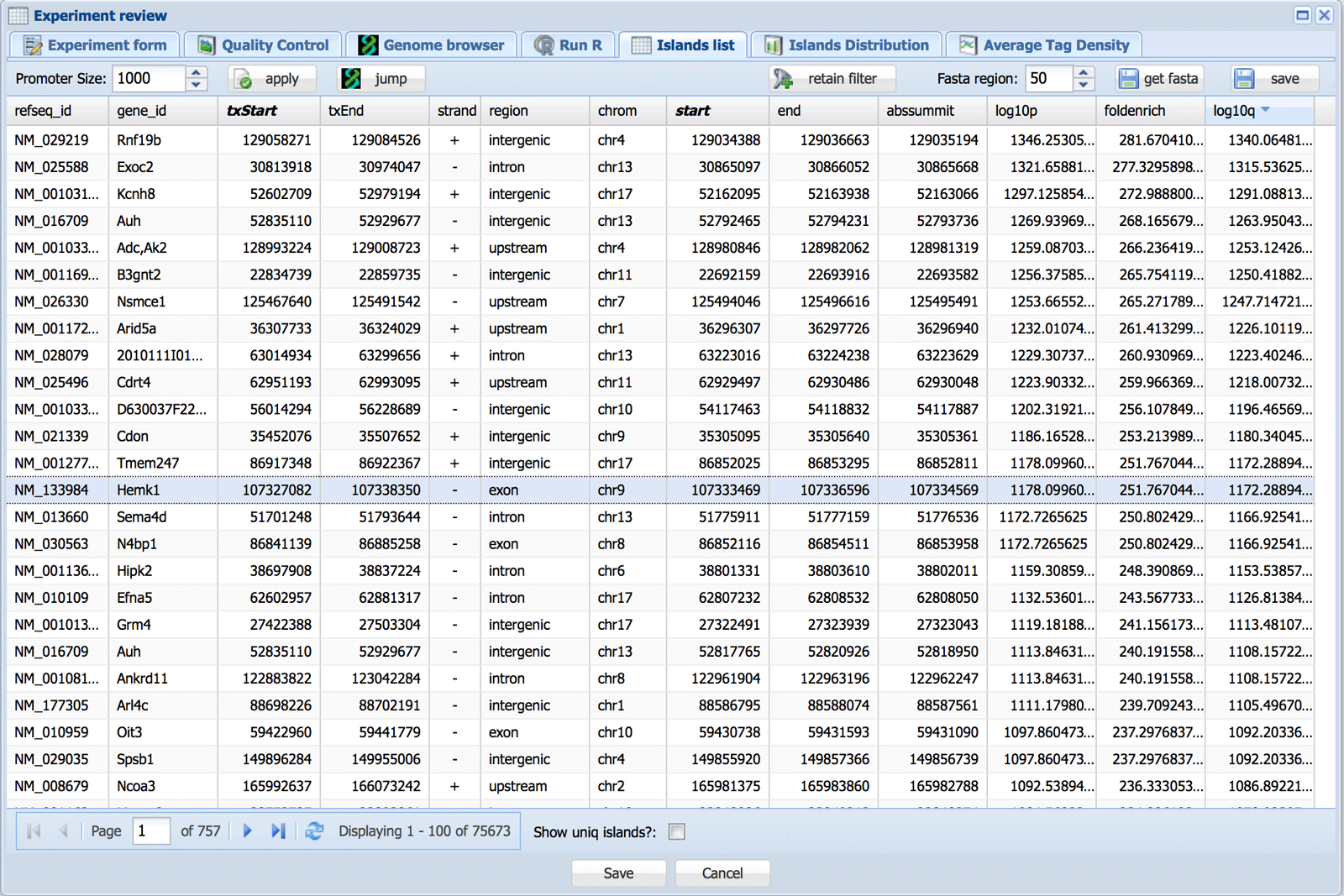
The Islands list tab appearss for DNA-Seq type records and shows the list of islands as detected by MACS2, statistics and the nearest gene. Islands are classified (“region” column) as intersecting with promoter, upstream (less than 20 kb), exon, intron or intergenic regions (in this order). The promoter radius can be adjusted; click the “apply” button after changes in the promoter size are made. This will also modify the peak distribution plot in the Island Distribution tab (see below).
If an island has multiple “summits” each summit coordinate (“start” and “end”) is shown as a separate row together with the position of the whole island (“txStart” and “txEnd”). Checking the “Show uniq islands?” box will show each island (start and end position; “txStart” and “txEnd”) only once and will not show summits. The “Jump” button opens the genome browser tab on the selected island. The “Save” button allows the table to be downloaded in .csv format.
The headings of the table can be used to filter peaks: e.g. selecting peaks with q value better than a certain threshold or 10000 best peaks, etc. This selection can be saved using the retain filter button and will be used in downstream analysis e.g. MAnorm.
The “get fasta” button can be used to obtain sequence located within X bases around each summit in the selected peaks. This can be used to obtain sequence logos with MEME-ChIP or MelinaII. Please note that Mac/Unix and Windows use different “End of Line” symbols. For this reason the sequences will not look properly fasta formatted in Windows. However, MEME will still recognize the format.
http://meme.nbcr.net/meme/doc/meme-chip.html
http://melina2.hgc.jp/public/index.html
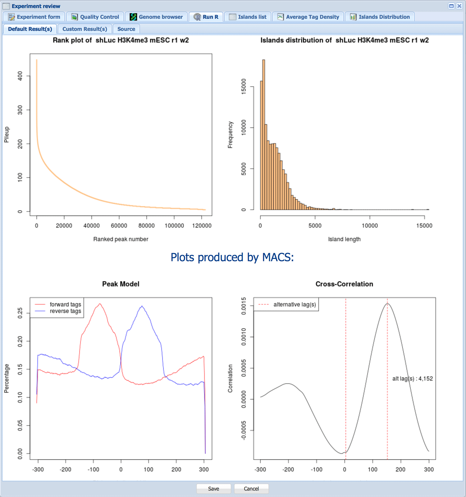
R tab was included to allow for easy integration of specialized tools into Wardrobe. It can be used to run R code within Wardrobe. Currently default code creates pileup vs. peak rank graphs and peak length histogram for ChIP-Seq. Additionally, this window is used to output plots produced by MACS.

For RNA-Seq, the default R code creates gene body coverage and RPKM histogram.
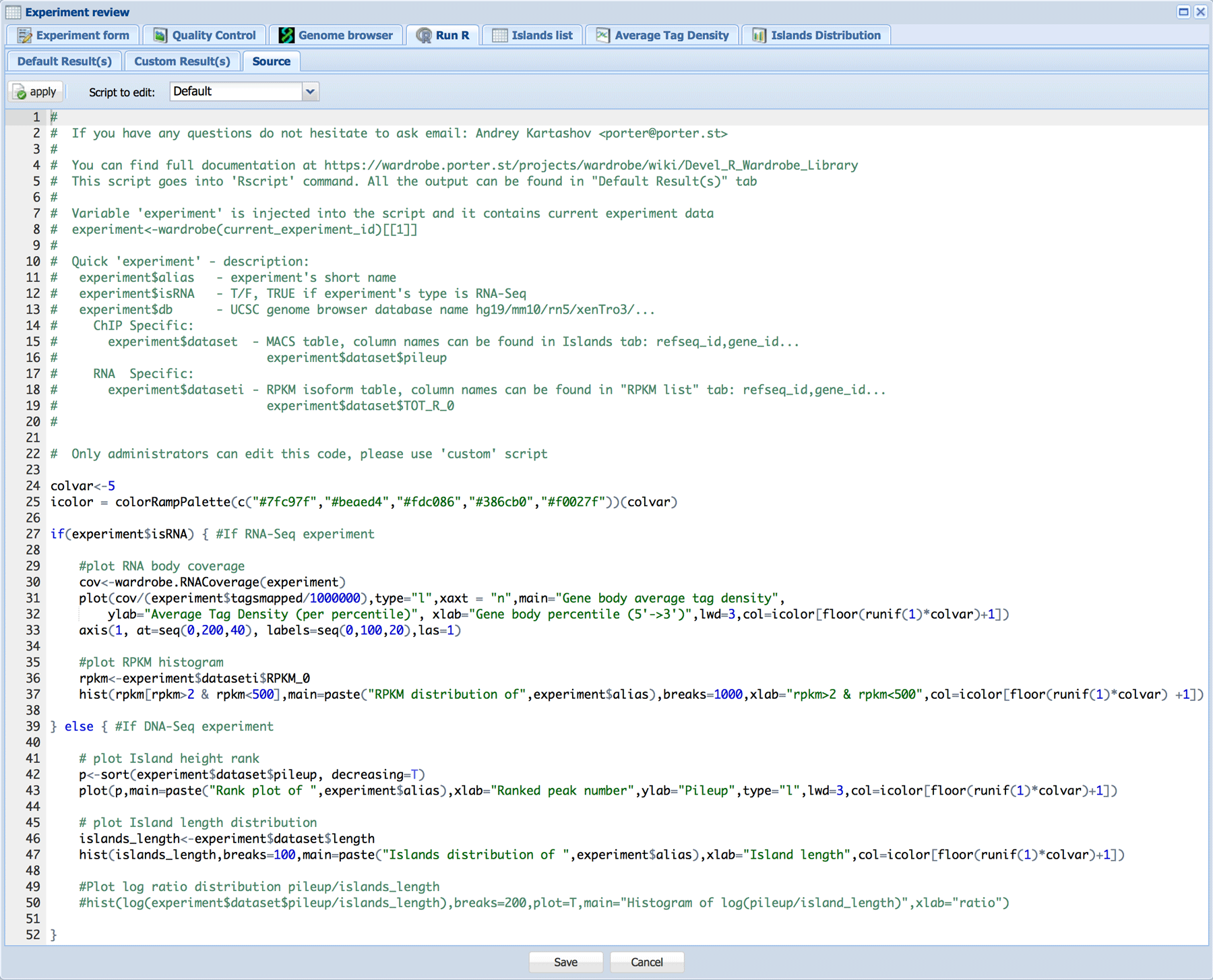
Custom R code can be edited by administrators in the Source tab. Please see help file for the Wardrobe R library for reference.

The Average Tag Density tab displays for DNA-Seq type records and shows the average tag density profile around all annotated TSS. Such graphs can be used to estimate the success of ChIP-Seq type experiments for some histone modifications (e.g. H3K4me).
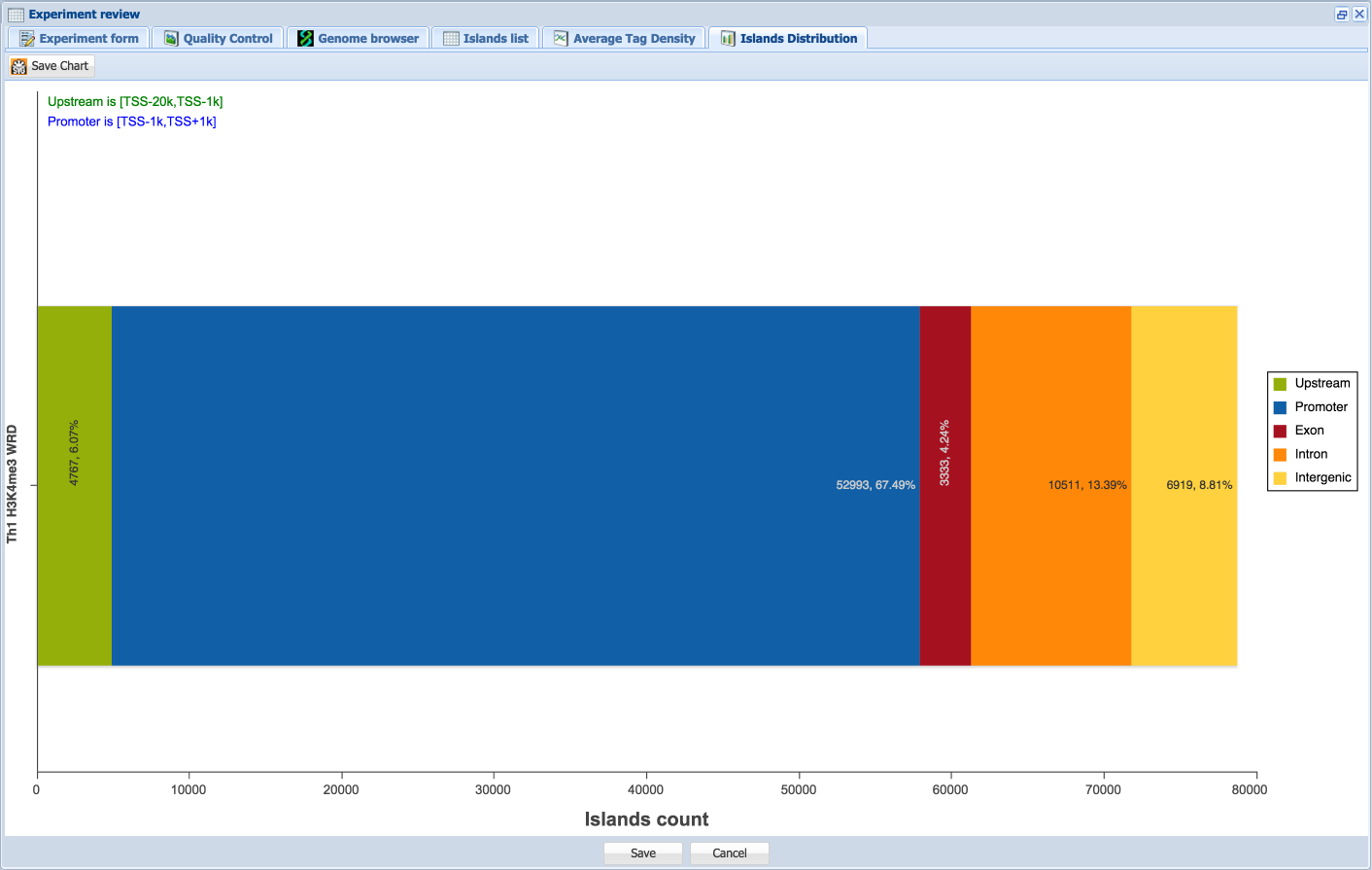
The Islands Distribution tab displays for DNA-Seq type records and shows distribution of islands between upstream, promoter, exon, intron and intergenic regions (in this order left to right). Area definitions in relation to the TSS are shown above the diagram for the upstream and promoter regions. The number and percentage of island counts per region are shown on each region in the diagram.