R scripts for Kleborate and Kaptive analysis
Here is a quick tutorial to calculate rapid raw and outbreak-adjusted proportions in your Kleborate data! This can even be performed in your terminal of choice if you want to quickly eyeball your data after a Kleborate run or PathogenWatch collection creation.
For a tutorial on how to create a PathogenWatch collection, please see the klebgenomics readme, the Klebsiella Sero-epi Shiny App or the PathogenWatch website.
In this example, I have downloaded both the Kleborate output and distance matrix from my PathogenWatch collection.
We will first load Kleborate functions for loading a single or multiple Kleborate files generated from either the the command-line version of Kleborate or Pathogenwatch.
source("https://raw.githubusercontent.com/klebgenomics/KleborateR/main/kleborate_functions.R")kleborate <- read_kleborate_file("pathogenwatch_kleborate.csv")Or if the data is from a URL...
kleborate <- read_kleborate_file("kleborate_data_maybe_from_figshare_or_github_raw_url.csv")Or if you have multiple CSVs from different runs...
kleborate <- read_kleborate_files(fs::dir_ls(glob="kleborate_*.csv"))Let's load in the cluster functions from this repo.
source("https://raw.githubusercontent.com/klebgenomics/KleborateR/main/cluster_functions.R")Now I'll read in my SNP distance matrix and calculate clusters using the default SNP distance threshold of 10. This will add a 'Cluster' column to the Kleborate data to indicate which genomes belong to the same cluster.
snps <- read_snp_diff("pathogenwatch_snp_dist.csv")
data <- get_cluster_membership_from_distmat(kleborate, snps)
I can optionally change the SNP distance threshold to 20 like so:
snps <- read_snp_diff("pathogenwatch_snp_dist.csv")
data <- get_cluster_membership_from_distmat(kleborate, snps, snp_dist=20)
Or just do in a one-liner:
data <- get_cluster_membership_from_distmat(readr::read_csv("pathogenwatch_kleborate.csv"), read_snp_diff("pathogenwatch_snp_dist.csv")) The data can have additional columns of metadata for performing adjusted counts such as "Country", "Site" and "Year". You can name them however you wish, but you MUST declare your cluster adjustment and epidemiological columns in the downstream functions.
Let's add a bit more metadata for cluster adjustment.
isolates_from_site1 <- c("a", "b", "c")
isolates_from_site2 <- c("x", "y", "z")
isolates_from_2009 <- c("a", "b", "c")
isolates_from_2010 <- c("x", "y", "z")

data <- data |>
 dplyr::mutate(
  Country = "United Kingdom",
  Site = dplyr::case_when(
   `Genome Name` %in% isolates_from_site1 ~ "Site1",
   `Genome Name` %in% isolates_from_site2 ~ "Site2",
   TRUE ~ "Site3"
  ),
  Year = dplyr::case_when(
   `Genome Name` %in% isolates_from_2009 ~ 2009,
   `Genome Name` %in% isolates_from_2010 ~ 2010,
   TRUE ~ 2011
  ),
 )
Now we have a bit more epidemiological information to adjust our proportions.
Let's load in the Kleborate functions from this repo.
source('https://raw.githubusercontent.com/klebgenomics/KleborateR/main/kleborate_functions.R')Let's look at the raw and outbreak-adjusted proportions of the K-locus.
get_counts(data, "K_locus")Which displays the following:
Removing K_locus from epi_vars
Grouping var: K_locus
Epi vars: ST, K_type, O_locus, O_type, Country, Study, Site, Cluster, Large_cluster
Adj vars: Cluster, Site, Study, ST
# A tibble: 140 × 14
   K_locus raw_count adj_count raw_prop adj_prop  n_ST n_K_type n_O_locus
   <chr>       <int>     <int>    <dbl>    <dbl> <int>    <int>     <int>
 1 KL107         731       448   0.0771   0.0710   197        1        12
 2 KL2           575       347   0.0606   0.0550    42        1         3
 3 KL102         721       309   0.0760   0.0490    38        1         4
 4 KL24          391       288   0.0412   0.0456    35        1         3
 5 KL15          368       189   0.0388   0.0300    31        1         2
 6 KL62          280       185   0.0295   0.0293    41        1         2
 7 KL25          248       182   0.0261   0.0288    36        1         5
 8 KL30          227       153   0.0239   0.0242    51        1         3
 9 KL28          175       148   0.0185   0.0235    31        1         5
10 KL17          232       148   0.0245   0.0235    15        1         4
# ℹ 130 more rows
# ℹ 6 more variables: n_O_type <int>, n_Country <int>, n_Study <int>,
#   n_Site <int>, n_Cluster <int>, n_Large_cluster <int>
# ℹ Use `print(n = ...)` to see more rows
Now, let's look at the raw and outbreak-adjusted proportions of each K-locus withn each ST.
raw_adj_prop(data, c("ST", "K_locus"))Which displays the following:
grouping_var: ST in adj_vars, removing from adj_vars
Grouping vars: ST, K_locus
Denominator: ST
Adj vars: Cluster, Site, Study
# A tibble: 1,973 × 6
   ST    K_locus raw_count adj_count raw_prop adj_prop
   <chr> <chr>       <int>     <int>    <dbl>    <dbl>
 1 ST307 KL102         562       189    0.988    0.964
 2 ST23  KL1           126       114    1        1
 3 ST101 KL17          193       113    0.877    0.856
 4 ST15  KL24          147       111    0.298    0.365
 5 ST15  KL112         222       111    0.449    0.365
 6 ST45  KL24          142       100    0.587    0.571
 7 ST14  KL2           157        96    0.720    0.686
 8 ST512 KL107         252        83    1        1
 9 ST20  KL28           79        76    0.669    0.667
10 ST17  KL25           97        71    0.439    0.452
The output is arranged by adj_count in descending order and the default denominator is the first
variable in the vector (in this case, ST). We can make the denominator "ST" by changing the
order of the vector to c("K_locus", "ST") OR by using the denominator argument:
raw_adj_prop(data, c("ST", "K_locus"), denominator="K_locus").
From this output preview, we can see that 100% of ST23 isolates have a KL1 capsule (K) locus, consistent with published data.
Now, let's plot this data!
Let's load in the plotting functions from this repo.
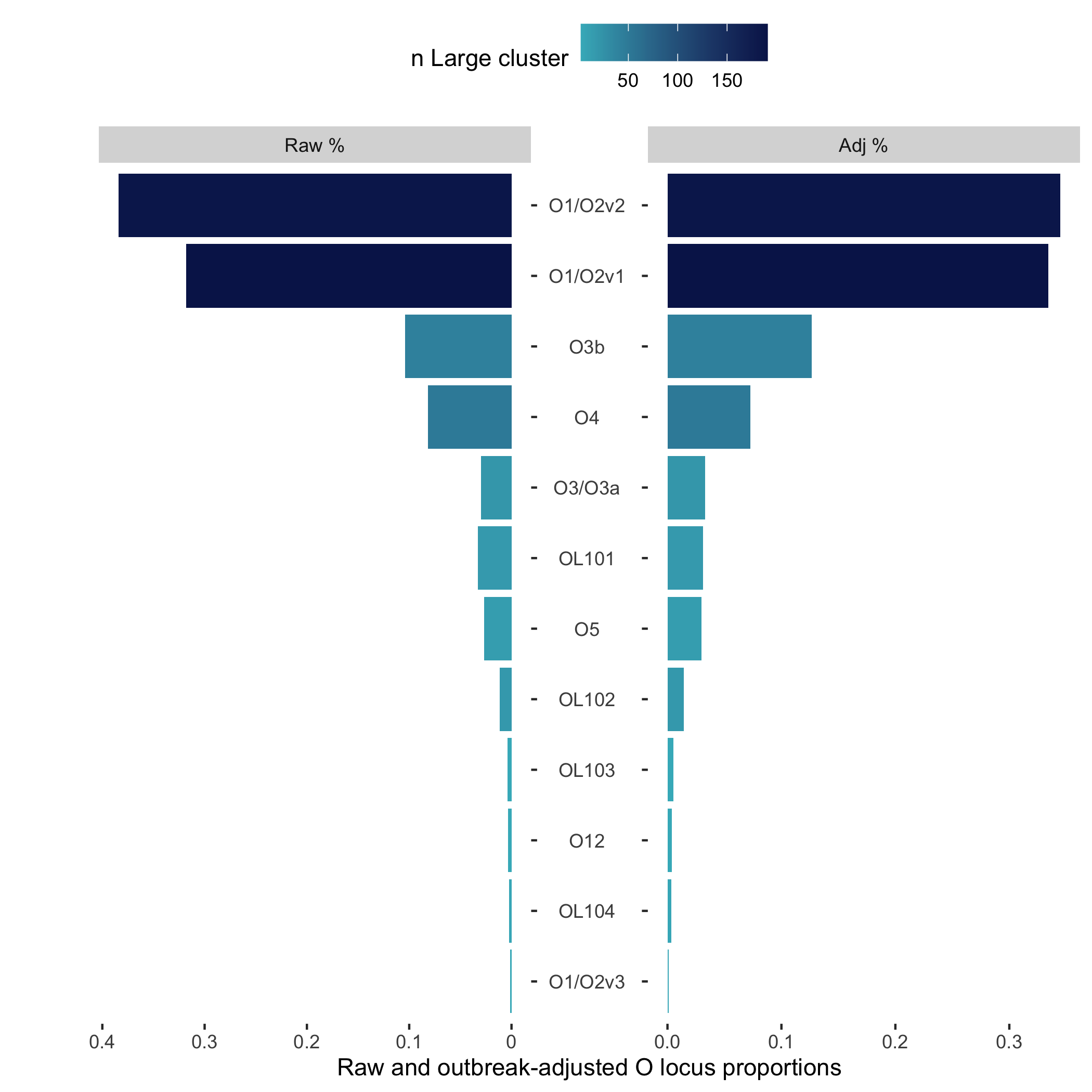
source('https://raw.githubusercontent.com/klebgenomics/KleborateR/main/plotting_functions.R')Let's plot the raw and outbreak-adjusted proportions of the O-loci in this data.
We can provide the get_counts output as an argument, or use a pipe like so!
get_counts(data, "O_locus") |> plot_raw_adj_pyramid()Which outputs the following plot: