INSY 695 - Enterprise Data Science

Team: Cloud Computations

Topic: Weather Prediction: A Case Study on Montreal, Quebec

Team Members:

• Richard Gao -- 260729805
• Jake Hogan -- 260731171
• Steven Liang -- 260415672
• Hanna Swail -- 260746086
• Duncan Wang -- 260710229

Introduction

The ability to produce accurate weather forecasts remains a crucial social and economic priority, with benefits cascading across sectors including transportation, tourism, and agriculture. The US Weather Service estimates that investment in public weather forecasts has an annualized benefit of over $31 billion (Lazo et al. 2009).

Classical approaches to weather forecasting by meteorologists use complex climatological models constructed from data collected from a large range of sources, from weather stations, to balloons, to radar and satellites. Because of this, access to good forecasts can be geographically constrained. While these models have been successful, there is still a significant opportunity for machine and deep learning models to improve the accuracy and geographic availability of traditional weather forecasting.

Objective

The objective of this project is to use historical time-series data to predict future average hourly and daily temperatures (in Celcius) in Montreal, explain what factors are driving local weather patterns, and see how our forecasts compare to the accuracy of current forecasts. We will be exploring several parametric, machine learning, and deep learning models, and comparing their relative performances. We will also use causal inference methods to examine driving factors, and utilize exogenous data streams and anomaly detection methods to improve prediction accuracy.

Hypotheses

We form the following 3 hypotheses:

1. Simple parametric models such as ARIMA will have a lower prediction error than more complicated machine learning or neural network models when given just past temperature patterns as a predictor to forecast future temperatures with (with no exogenous variables)
2. Neural Network models will perform best when a large variety of predictors are available, since they are generally more capable of identifying and capturing any hidden variable relationships, when present, that might not be visible to the human eye.
3. The best explanatory factor for temperature will simply be the most recent available past temperatures.

Table of Contents:

Section 1: Data Preparation

Section 2: Parametric Models

Section 3: Machine Learning Models

Section 4: Neural Network Models

Section 5: AutoML

Section 6: Causal Inference

Section 7: Deployment

Important Notebooks:

• Parametric Models
• Machine Learning Models
• AutoML Models
• Causal Inference
• Presentation Deck
• RNN Daily Aggregation
• Anomaly Detection Daily Aggregate
• EDA
• Feature Engineering

Data Source

Access the data here

Methods

Section 1: Data Preparation

• Data extraction

• Data cleansing & preprocessing

• EDA

Descriptive weather events versus temperature

Feature histograms broken down by weather events

Hourly, monthly, weekly Trend analysis

Daily Temperature plot brokwn down by actual, minimum and maximum

• Feature Engineering:
  • time point extraction,
  • lagged features,
  • [max,min,average]X[daily,weekly,monthly]X[temp,humidity,wind direction/speed] from the previous time point
    • ie. max daily temp, min daily temp, average daily temp, max weekly temp, min weekly temp,...etc
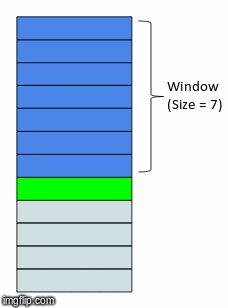
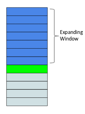
  • rolling and expanding window

Rolling Window

Expanding Window

• Feature Selection using RFE

Sample RFE output

Section 2: Parametric Models

• Autoregressive Integrative Moving Average (ARIMA)
• Generalized Additive Model

Seasonal ARIMA

A seasonal ARIMA model was built using a process of gridsearch to determine the optimal seasonal and non-seasonal ARIMA Autoregression (A), Integration (I), and Moving Average (MA) parameters required. The simple ARIMA achieved a MAE of 2.57.

Generalized Additive Model The Generalized Additive Model was built using Facebook's forecasting tool, Prophet, which achieved an MAE of 3.75. We see this case that ARIMA performs better, as it appears to fit the daily fluctuations better than the GAM model, which generalizes the pattern but misses the ups and downs. We propose this could because GAM uses a sum of smooth functions & a process of backfitting to fit a trend line.

Section 3: Machine Learning Models

A variety of Machine Learning models were fit, using both a simple set of features consisting of different combinations of the lagged past values of temperature and time components, as well as a more complex set of features including humidity, windspeed, and wind direction. We also performed Bayesian hyperparameter optimization using Hyperopt to further tune the models. Overall, XGBoost was best at identifying important predictors and benefited from the information given by a more comprehensive feature set, but hyperparameter tuning had little to no effect on the model. The best XGBoost model with an increased feature set obtained an MAE of 2.42, but the simple XGBoost model performed worse, with an MAE of 2.77.

SHAP Analysis: We also used SHAP for feature importance interpretation:

Initial Summary: Lag1 is are most important predictor (consistent with regular feature importance)

Depedence Plots:

• We see the strong direct linear proportional relationship lag1 and predictions

We can also see where it start to diverge, if we looked at lag12 for instance

• The relationship is similar but is not as strong
• There are a lot more outliers
• Especially with low lag12 temperatures can be associated with a big range of low to high temperature predictions

Whether we added more or less features, lag1 stayed the #1 predictor.

Section 4: Neural Network Models

Results contained within the RNN Daily Aggregation notebook and the Anomaly Detection Daily Aggregate notebook. The LSTM and Transformer models are created and tested in RNN Daily Aggregation. Autoencoders and anomaly detection are contained within the Anomaly Detection Daily Aggregate notebook.

• LSTM
• Transformers
• Anomaly detection using Autoencoders

Section 5: AutoML

We also compared our RNN results with an RNN AutoML model built using Ludwig, which obtained a MAE of 2.85.

Section 6: Causal Inference (DoWhy)

There was a lot of experiemntation with this section as our initial results were pretty strange looking and distorted. We see that overall, there's not that much of an impact at all from our regular features we fed into the ML models. We believe that there are a few issues that are causing this:

• Due to the nature of our project, the data we are working with comes with specific data profiles such as temperature being cyclical and also features such as humidity, windspeed/direction, pressure exist in all types of temperature ranges...leading to a causal result that's near zero.

• We have many feature that are engineered. Here we are using what we fed into some of our initial model trial runs, and we see that with causal inference, it's not easy to interpret. While this is the initial test, subsequent test will have to be more narrow in terms of what we want to see and push into DoWhy. We will be choosing our features more carefully and also be more mindful of feature engineering for specific features.

Inital Results :

Final Results - Through careful feature selection and engineering

• Creation of seasons variables for intperpreability
• Changing continous variables like pressure, wind speed and humidity into categorical low, medium and high categories through quanitiles.
• Dropping the medium category to keep the data with the highest variance.

These results above look much better in terms of treatment effects on temperature.

• High Pressure = cold vs Low Pressure
• High Humidity = warmer vs low humidity
• Wind Speed = no difference high vs low

Other Insights:

• Autume is warmer than spring
• Winter = cold, Summer = hot

• While "Winter = cold, Summer = hot" might seem like a no brainer to us, keep in mind that keep in mind that a computer doesn't know what the concept summer and winter is, and that seeing results that we know are good is not something we should take for granted. If anything it goes back to the trust and transparency topic we covered a while back - seeing obvious results give confidence for other insight the model provides which are good.

Weather Patterns on Temperature:

• Snow is causes with cooler temperatures
• Thunderstorms cause warmer temperatures
• Most other weather patterns are on the warm side too.

Which makes sense for precipitation.

Section 7: Deployment

We created a dashboard that queries the fastapi (localhost:8000)

We created a fastapi, everytime our dockerfile is run, it is packaged as a docker container and is hosted on AWS ECR/ECS. You can also run using uvicorn after installing the requirements.txt. The contents are stored in Cloud-Computations folder under the src folder.

We tracked or model every time it was built. You can run using the command: mlflow server --backend-store-uri sqlite:///mlflow.db --default-artifact-root ./artifacts --host 0.0.0.0

You can run the deploy.sh script in order to generate a docker image. Our use our Jenkins file to build a CI/CD pipeline.

Conclusion and Next Steps

In conclusion, we proved that the best explanatory variables were indeed past temperature. However, neural networks did not perform best with a large variety of predictors. We did find though, that adding features to the XGBoost model did improve performance a bit. Lastly, the ARIMA model outperform XGBoost as we had originally thought, with a simple set of features, but XGBoost performed the best overall since it was more easily able to take advantage of a larger set of features. To conclude, the major threats to our model formulation is applying it to different locations, as geographical region can have a large impact on variable interactions. In our next steps, we would like to test the models and explore causal inference for different cities and quantify to what degree having multiple models for different cities is indeed beneficial (relative to a single model applied to all). We would also like to explore multi step forecasting for long-range forecasting purposes.